본 포스팅에서는 로지스틱 회귀 기반 심층신경망 학습을 진행해보겠습니다.
로지스틱 회귀는 선형 회귀와 비슷하나 직선 대신 S자 곡선을 이용하여 분류의 정확도를 향상한 방법입니다.
특정 값의 변화를 예측, 이진 분류에 사용됩니다.
아래 코드는 이진 분류이며, 은닉층을 증가시킨 신경망을 이용했습니다.
참고 : wikidocs.net/111476
# 단순한 로지스틱 회귀 예제 (텐서플로우2)
import numpy as np
import matplotlib.pyplot as plt
import tensorflow as tf
from sklearn.model_selection import train_test_split
# x(입력), y(결과) 데이터
x_train = np.array([-50, -40, -30, -20, -10, -5, 0, 5, 10, 20, 30, 40, 50,
-15, 1, 3, -7, 2.5,
7, 77, 33, 52, 80])
y_train = np.array([0, 0, 0, 0, 0, 0, 0, 0, 1, 1, 1, 1, 1,
0, 0, 0, 0, 0,
1, 1, 1, 1, 1])
# train 데이터와 test 데이터로 분리 (80:20)
x_train, x_test, y_train, y_test = train_test_split(x_train, y_train, test_size=0.2, random_state=77)
# keras의 다차원 계층 모델인 Sequential를 레이어를 만든다.
model = tf.keras.models.Sequential()
# 입력이 1차원이고 출력이 1차원임을 뜻함 - Dense는 레이어의 종류
model.add(tf.keras.layers.Dense(5, input_dim=1))
model.add(tf.keras.layers.Dense(3))
model.add(tf.keras.layers.Dense(1, activation='sigmoid'))
# 종합
model.summary()
# Optimizer: Stochastic gradient descent (확률적 경사 하강법)
sgd = tf.keras.optimizers.SGD(learning_rate=0.01)
# Loss function: binary_crossentropy (이진 교차 엔트로피)
model.compile(optimizer=sgd, loss='binary_crossentropy', metrics=['binary_accuracy'])
# 주어진 X와 y데이터에 대해서 오차를 최소화하는 작업을 200번 시도합니다.
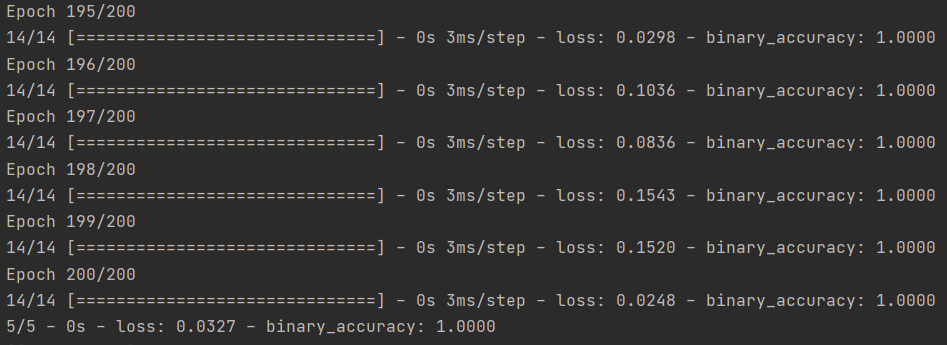
hist = model.fit(x_train, y_train, batch_size=1, epochs=200, validation_split=0.2)
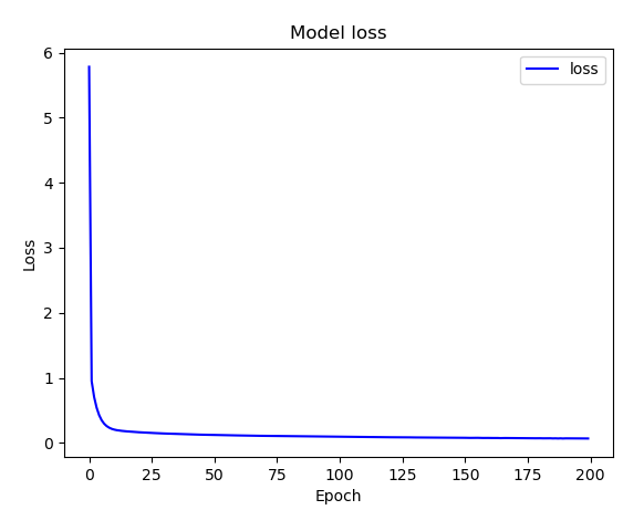
# 모델 손실 함수 시각화
plt.plot(hist.history['loss'], 'b-', label='loss')
plt.title('Model loss')
plt.xlabel('Epoch')
plt.ylabel('Loss')
plt.legend()
plt.show()
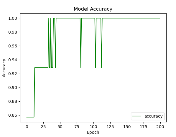
# 모델 정확도 시각화
plt.plot(hist.history['binary_accuracy'], 'g-', label='accuracy')
plt.title('Model Accuracy')
plt.xlabel('Epoch')
plt.ylabel('Accuracy')
plt.legend()
plt.show()
# 손실 함수 계산
model.evaluate(x_test, y_test, batch_size=1, verbose=2)
# 모델 시각화
line_x = np.arange(min(x_test), max(x_test), 0.01)
line_y = model.predict(line_x)
plt.plot(line_x, line_y, 'r-')
plt.plot(x_test, y_test, 'bo')
plt.title('Model')
plt.xlabel('test')
plt.ylabel('predict')
plt.legend(['predict', 'test'], loc='upper left')
plt.show()
# 모델 테스트
print(model.predict([1, 2, 3, 4, 4.5]))
print(model.predict([11, 21, 31, 41, 500]))
코드를 분석해보면,
선형 회귀와 거의 유사하지만 몇 가지 다른점이 있습니다.
먼저 이진 분류이기 때문에 정답이 0, 1 두 가지로 구성됩니다.
이진 분류를 위해서는 데이터를 0과 1사이의 값으로 변환하는 것이 표현하기 좋기 때문에 활성화 함수는 시그모이드 함수를 사용했습니다.
옵티마이저는 선형 회귀와 똑같이 확률적 경사 하강법을 사용했으며, 손실 함수는 바이너리 크로스 엔트로피를 사용했습니다.
시그모이드 함수는 곡선 형태이기 때문에, 경사 하강법에서 미분값이 0이 되는 점은 1개 이상일 수 있습니다. (극솟값)
따라서 교차 엔트로피 함수를 통해 극솟값이 최솟값이 될 수 있도록 합니다.
fit()을 이용하여 학습을 진행합니다. 정확도는 100 epoch 정도에서 1.0으로 고정되며 손실도는 0.1~0.3사이로 수렴합니다.
손실 함수를 시각화합니다.
정확도를 시각화합니다.
학습 데이터와 예측 값을 비교해봅니다. S자 형태의 곡선으로 시그모이드 함수의 모양을 띄고 있습니다.
대부분 곡선위에 점이 존재하고 있습니다. (잘 학습됨)
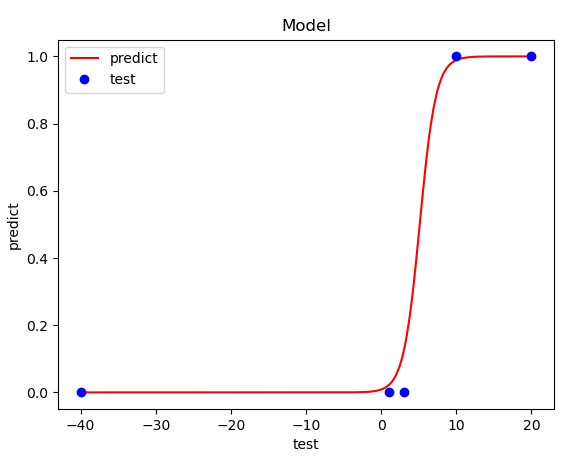
로지스틱 회귀를 이용한 이진 분류에서 임계치는 0.5입니다.
학습한 모델에 실제 데이터를 입력하여 예측해봅니다.
학습 데이터를 기준으로 10미만의 실수는 '0'으로 분류하고, 10이상의 실수는 '1'로 분류합니다.
임계값 0.5를 기준으로 '0', '1'로 분류할 수 있습니다.
print(model.predict([1, 2, 3, 4, 4.5]))
print(model.predict([11, 21, 31, 41, 500]))

'AI > TensorFlow & PyTorch' 카테고리의 다른 글
| [TensorFlow] 텐서플로우(TensorFlow 2.x) 와인 데이터 다항 분류 (0) | 2021.03.05 |
|---|---|
| [TensorFlow] 텐서플로우(TensorFlow 2.x) 와인 데이터 이항 분류 (0) | 2021.03.05 |
| [TensorFlow] 텐서플로우(TensorFlow 2.x) 보스턴 주택 가격 예측 (0) | 2021.03.02 |
| [TensorFlow] 텐서플로우(TensorFlow 2.x) 선형 회귀 예제 (0) | 2021.02.26 |
| [TensorFlow] 텐서플로우(TensorFlow 2.x) 개발 환경 구축 (Windows) (1) | 2021.02.22 |