이전 포스팅에서 Fashion MNIST 데이터를 DNN을 이용해 학습했습니다.
이번에는 CNN을 이용하여 학습해보겠습니다.
코드는 '텐서플로 2.0 프로그래밍' 예제에서 가져왔습니다.
import tensorflow as tf
import matplotlib.pyplot as plt
# set gpu
gpus = tf.config.experimental.list_physical_devices('GPU')
if gpus:
try:
# Currently, memory growth needs to be the same across GPUs
for gpu in gpus:
tf.config.experimental.set_memory_growth(gpu, True)
logical_gpus = tf.config.experimental.list_logical_devices('GPU')
print(len(gpus), "Physical GPUs,", len(logical_gpus), "Logical GPUs")
except RuntimeError as e:
# Memory growth must be set before GPUs have been initialized
print(e)
# 6.4 Fashion MNIST 데이터셋 불러오기 및 정규화
fashion_mnist = tf.keras.datasets.fashion_mnist
(train_X, train_Y), (test_X, test_Y) = fashion_mnist.load_data()
train_X = train_X / 255.0
test_X = test_X / 255.0
# 6.5 데이터를 채널을 가진 이미지 형태(3차원)으로 바꾸기
# reshape 이전
print(train_X.shape, test_X.shape)
train_X = train_X.reshape(-1, 28, 28, 1)
test_X = test_X.reshape(-1, 28, 28, 1)
# reshape 이후
print(train_X.shape, test_X.shape)
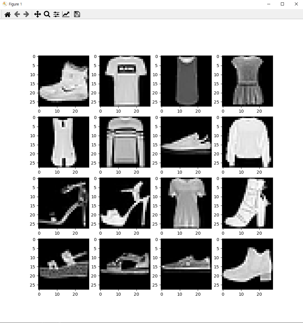
# 6.6 데이터 확인
# 전체 그래프의 사이즈를 width=10, height=10 으로 지정합니다.
plt.figure(figsize=(10, 10))
for c in range(16):
# 4행 4열로 지정한 grid 에서 c+1 번째의 칸에 그래프를 그립니다. 1~16 번째 칸을 채우게 됩니다.
plt.subplot(4, 4, c + 1)
plt.imshow(train_X[c].reshape(28, 28), cmap='gray')
plt.show()
# train 데이터의 첫번째 ~ 16번째 까지의 라벨을 프린트합니다.
print(train_Y[:16])
# 6.7 Fashion MNIST 분류 컨볼루션 신경망 모델 정의
model = tf.keras.Sequential([
tf.keras.layers.Conv2D(input_shape=(28, 28, 1), kernel_size=(3, 3), filters=16),
tf.keras.layers.Conv2D(kernel_size=(3, 3), filters=32),
tf.keras.layers.Conv2D(kernel_size=(3, 3), filters=64),
tf.keras.layers.Flatten(),
tf.keras.layers.Dense(units=128, activation='relu'),
tf.keras.layers.Dense(units=10, activation='softmax')
])
model.compile(optimizer=tf.keras.optimizers.Adam(),
loss='sparse_categorical_crossentropy',
metrics=['accuracy'])
model.summary()
# 6.9 Fashion MNIST 분류 컨볼루션 신경망 모델 학습
history = model.fit(train_X, train_Y, epochs=25, validation_split=0.25)
plt.figure(figsize=(12, 4))
plt.subplot(1, 2, 1)
plt.plot(history.history['loss'], 'b-', label='loss')
plt.plot(history.history['val_loss'], 'r--', label='val_loss')
plt.xlabel('Epoch')
plt.legend()
plt.subplot(1, 2, 2)
plt.plot(history.history['accuracy'], 'g-', label='accuracy')
plt.plot(history.history['val_accuracy'], 'k--', label='val_accuracy')
plt.xlabel('Epoch')
plt.ylim(0.7, 1)
plt.legend()
plt.show()
model.evaluate(test_X, test_Y, verbose=0)컨볼루션 연산은 굉장히 복잡하기 때문에, GPU를 사용하고 있을 경우 set_memory_growth()를 통해 VRAM의 공간 제한을 없애줘야 합니다.
Fashin MNIST의 데이터는 크기가 28x28인 흑백 이미지입니다. RGB 채널은 3이지만, 흑백은 1이기 때문에 reshape()를 이용하여 채널을 추가합니다.
이후 reshape()한 데이터를 확인합니다.
Sequential()을 이용하여 높이 28, 너비 28, 채널 1인 컨볼루션 레이어를 생성합니다.
총 3개의 컨볼루션 레이어를 생성하는데 필터의 수는 16을 시작으로 2배씩 증가시켰습니다. (개인 설정)
필터의 크기는 모두 3x3으로 설정했습니다.
옵티마이저는 Adam을, 손실 함수는 다중 분류 손실 함수(sparse_categorical_crossentropy)를 사용했습니다.
25%는 테스트 데이터로 분리하고, 25번의 반복을 진행했습니다.
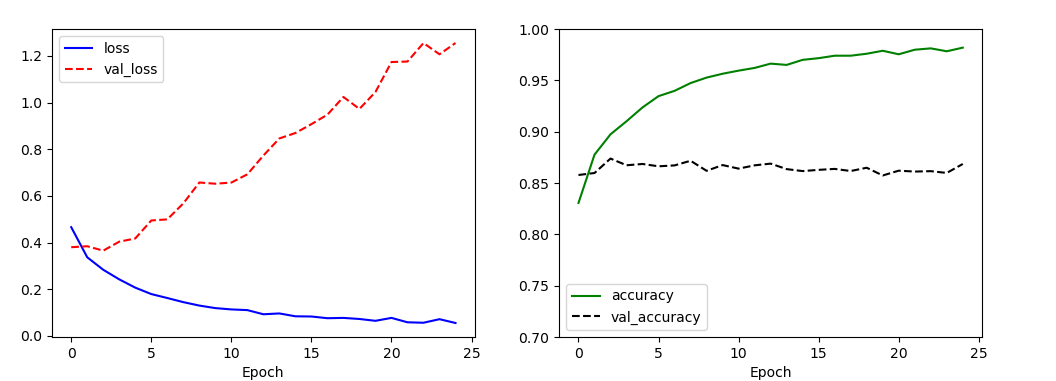
테스트 데이터의 정확도는 약 85%입니다. DNN을 이용하는 것보다 적은 수치입니다.
이를 개선하기 위해 풀링 레이어와 드롭아웃 레이어를 추가해보도록 하겠습니다.
# 6.10 Fashion MNIST 분류 컨볼루션 신경망 모델 정의 - 풀링 레이어, 드랍아웃 레이어 추가
model = tf.keras.Sequential([
tf.keras.layers.Conv2D(input_shape=(28,28,1), kernel_size=(3,3), filters=32),
tf.keras.layers.MaxPool2D(strides=(2,2)),
tf.keras.layers.Conv2D(kernel_size=(3,3), filters=64),
tf.keras.layers.MaxPool2D(strides=(2,2)),
tf.keras.layers.Conv2D(kernel_size=(3,3), filters=128),
tf.keras.layers.Flatten(),
tf.keras.layers.Dense(units=128, activation='relu'),
tf.keras.layers.Dropout(rate=0.3),
tf.keras.layers.Dense(units=10, activation='softmax')
])
model.compile(optimizer=tf.keras.optimizers.Adam(),
loss='sparse_categorical_crossentropy',
metrics=['accuracy'])
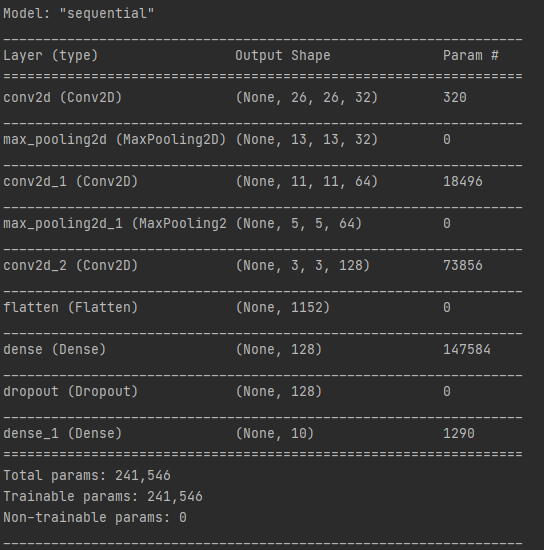
model.summary()
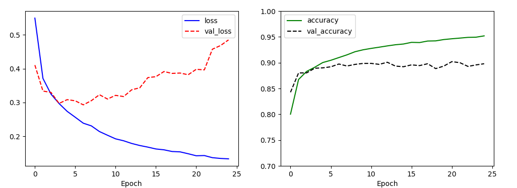
# 6.11 Fashion MNIST 분류 컨볼루션 신경망 모델 학습 - 풀링 레이어, 드랍아웃 레이어 추가
history = model.fit(train_X, train_Y, epochs=25, validation_split=0.25)
plt.figure(figsize=(12, 4))
plt.subplot(1, 2, 1)
plt.plot(history.history['loss'], 'b-', label='loss')
plt.plot(history.history['val_loss'], 'r--', label='val_loss')
plt.xlabel('Epoch')
plt.legend()
plt.subplot(1, 2, 2)
plt.plot(history.history['accuracy'], 'g-', label='accuracy')
plt.plot(history.history['val_accuracy'], 'k--', label='val_accuracy')
plt.xlabel('Epoch')
plt.ylim(0.7, 1)
plt.legend()
plt.show()
model.evaluate(test_X, test_Y, verbose=0)28x28x1 크기의 데이터를 콘볼루션 레이어의 입력으로 받습니다. 필터의 크기는 3x3이며, 필터의 개수는 32개입니다.
스트라이드는 생략되어 디폴트 값인 1x1 입니다.
즉, 첫 번째 컨볼루션 레이어의 출력은 26x26x32 입니다. (마지막 32는 필터 크기 32입니다.)
첫 번째 맥스 풀링 레이어의 스트라이드 크기가 2x2이므로, 출력은 13x13x32가 됩니다.
플래튼 레이어는 마지막 컨볼루션 레이어를 일렬로 펼친것으로, 출력은 3x3x128 = 1152가 됩니다.
신경망이 깊어질수록 시그모이드 함수를 사용할 경우 역전파 과정에서 그래디언트 배니싱 (경사 소실) 문제가 발생하기 때문에 드롭 아웃 레이어전에 덴스 레이어에서 활성화 함수로 렐루 함수를 사용합니다.
드롭 아웃 레이어에서 무작위로 가중치 부분 집합을 제거하는 비율은 0.3으로 설정했습니다.
마지막 덴스 레이어에서는 다중 분류를 위해 활성화 함수로 소프트맥스 함수를 사용했습니다.
옵티마이저와 손실 함수는 동일합니다.
풀링 레이어와 드롭 아웃 레이어를 모델에 추가했을 때, 이전 모델의 정확도보다 4% 증가한 85%의 정확도를 확인할 수 있습니다.
'AI > TensorFlow & PyTorch' 카테고리의 다른 글
| [TensorFlow] 오토 인코더를 이용한 이미지 노이즈 제거 (0) | 2023.06.08 |
|---|---|
| [TensorFlow] RNN, LSTM, GRU를 이용한 영화 리뷰 감성 분석 (0) | 2023.06.08 |
| [TensorFlow] This is probably because cuDNN failed to initialize 오류 (0) | 2021.04.06 |
| [TensorFlow] 텐서플로우(TensorFlow 2.x) Fashion MNIST (0) | 2021.03.05 |
| [TensorFlow] 텐서플로우(TensorFlow 2.x) 와인 데이터 다항 분류 (0) | 2021.03.05 |